Morse-Smale Systems

Information

This is the project for my Master's Degree at San Jose State University. The content of this project is highly technical and is not intended for the general readers. The committee members include:

Professor Slobodan Simic (advisor)
Professor Richard Kubelka (committee member)
Professor Samih Obaid (committee member)

Abstract

This project presents a brief survey of Morse-Smale systems. We focus on continuous-time dynamical systems, i.e., flows defined by smooth vector fields. A dynamical system is called Morse-Smale if:

It has finitely many equilibria and closed orbits, all hyperbolic.
The stable and unstable manifolds of the equilibria and closed orbits intersect transversely.
The nonwandering set consists only of equilibria and closed orbits.

We provide the background material necessary to state the main properties of Morse-Smale systems; namely, that they form an open set in the space of all dynamical systems, that they are structurally stable, and, in dimension two, that they are also dense. Furthermore, on compact surfaces, a system is structurally stable if and only if it is Morse-Smale. We do not provide proofs of these results but instead focus on some specific but illustrative cases. In particular, by an explicit construction we show how to approximate an irrational fow on the torus by a Morse-Smale system.

Introduction

The field of dynamical systems, which originated from classical Newtonian mechanics in the beginning of the 20 century, was first developed by Henri Poincaré (1854-1912). Started by his interest in studying the stability of the Solar System. Since solving differential equations explicitly is rarely possible, Poincaré encourages us to look at the problems qualitatively instead. Many other mathematicians followed his suggestions including:

Aleksandr Lyapunov (1857-1918): studied the stability of dynamical systems, generalized the determination of the asymptotic behavior of these equilibria.
George Birkhoff (1884-1944): proved Poincaré's "Last Geometric Theorem," a special case of the three-body problem.
Stephen Smale (1930): developed the Smale horseshoe

To investigate the behavir of dynamical systems as time goes to infinity, It is useful to investigate this behavior using some generic dynamical systems.

Kupka-Smale systems
Morse-Smale systems

For the purpose of demonstration, we will skip the preliminary definition and theorems. Please refer to the full article for more information.

Morse-Smale Vector Fields

Definition: A vector field $X \in \mathfrak{X}^r(M)$ on a compact manifold $M$ is a Morse-Smale vector field if:

There are only a finite number of critical elements (singularities and closed orbits) on $X$ and they are all hyperbolic.
For any two critical elements $\sigma_1$ and $\sigma_2$ of $X$, their stable and unstable manifolds are transverse to each other
$\Omega(X)$ is the union of all the critical elements of $X$.

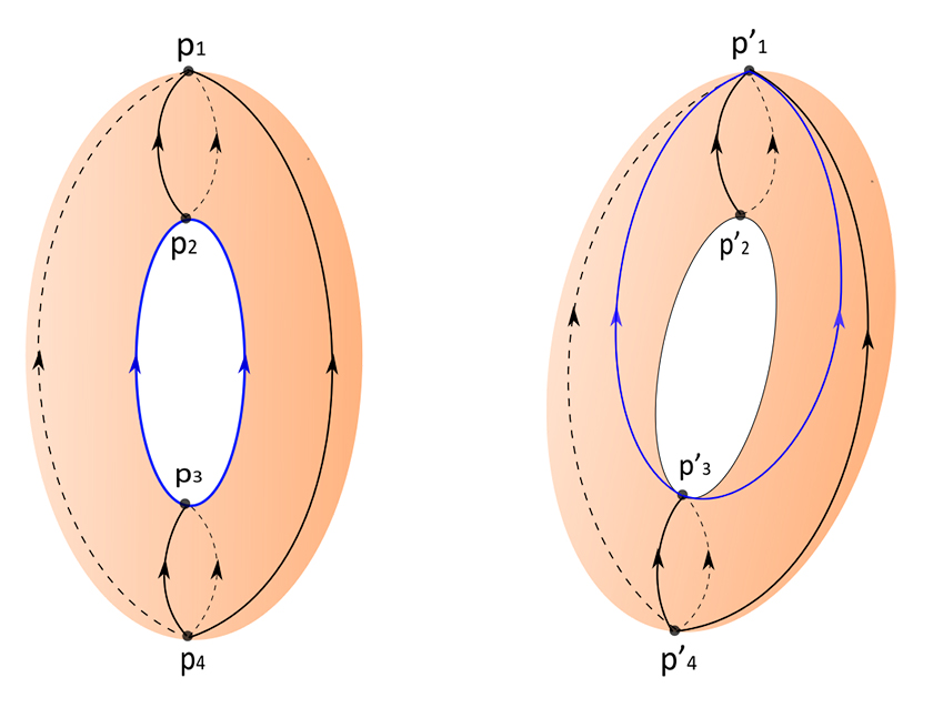
**Figure:** Examples of Kupka-Smale and Non-Kupka-Smale vector fields

In the example of the upright torus above, the vector field $X$ has four singularities: a source $p_4$, a sink $p_1$ and two saddles $p_2$ and $p_3$. The blue orbit represents both the stable manifold of $p_2$ and the unstable manifold of $p_3$. Since they are coincident, they do not intersect each other transversely, and they create an orbit connecting two saddles (a saddle connection). As a result, $X$ fails to be a Kupka-Smale vector field. However, a small perturbation can eliminate this saddle connection and change $X$ into a Kupka-Smale vector field $X'$. By tilting the torus slightly, the new singularities $p'_1,p'_2,p'_3$ and $p'_4$ will be very close to $p_1,p_2,p_3$ and $p_4$. However, we no longer have the old saddle connection as the unstable manifold of $p'_3$ now flows to the sink $p'_1$ (the red orbit). Thus, $X'$ is now a Kupka-Smale field. Morse-Smale vector fields will form a subclass of Kupka-Smale fields.

Definition: A point $p$ in $M$ is called a wandering point for a vector field $X$ if there exists a neighborhood $V$ of $p$ and a number $t_0>0$ such that $X_t(V) \cap V = \emptyset$ for $|t|>t_0$, where $X_t$ is the flow of $X$. Otherwise, $p$ is called a nonwandering point.

The set of all nonwandering points of $X$ is denoted by $\Omega(X)$.

Definition: A vector field $X \in \mathfrak{X}^r(M)$ on a compact manifold $M$ is a Morse-Smale vector field if:

There are only a finite number of critical elements (singularities and closed orbits) on $X$ and they are all hyperbolic.
For any two critical elements $\sigma_1$ and $\sigma_2$ of $X$, their stable and unstable manifolds are transverse to each other
$\Omega(X)$ is the union of all the critical elements of $X$.

Proposition: A vector field $X \in \mathfrak{X}^r(M)$ on a compact manifold $M$ is Morse Smale if and only if:

There are only a finite number of critical elements (singularities and closed orbits) on $X$ and they are all hyperbolic.
There are no saddle-connections.
Each orbit on $M$ has a unique critical element as its $\omega$-limit and a unique critical element as its $\alpha$-limit.

Let $X$ be a Morse-Smale vector field. The phase diagram of $X$ is the simplest way to represent the qualitative behavior of $X$.

**Figure:** Examples of phase diagrams of vector fields.

Strutural Stability of Morse-Smale Systems

In this section, we will look into an important property of Morse-Smale systems: structural stability.

Definition: A vector field $X \in \mathfrak{X}^r(M)$ is structually stable if there exists a $C^r$ neighborhood $U$ of $X$ such that for every vector field $Y$ in $U$, $Y$ is topologically equivalent to $X$.

To show that two vector fields $X$ and $Y$ are topologically equivalent to each other, we need to construct a homeomorphism that takes orbits of $X$ to orbits of $Y$.

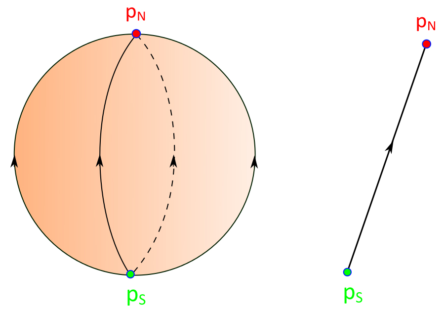
Theorem: Given a Morse-Smale vector field $X$ on $M$, there exists a neighborhood $U$ of $X$ such that for every vector field $Y \in U$, $Y$ is Morse-Smale and its phase diagram is isomorphic to that of $X$.

Theorem: If $X$ is a Morse-Smale vector field, then $X$ is structurally stable.

The complete proof of this theorem can be found in the full article. The proof for the North Pole-South Pole vector field can be outlined as followed:

By the previous theorem: there exists a neighborhood $U$ of $X$ such that for all $Y \in U$, $Y$ is Morse-Smale.
By the previous theorem: there exists an isomorphism $\sigma$ that takes the phase diagram of $X$ to the the phase diagram of $Y$.
Let $\psi_t$ be the flow by $X$ and $\varphi_t$ be the flow by $Y$.

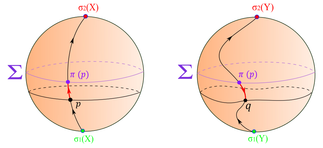
Next, we construct a homeomorphism $h: M \rightarrow M$ that takes orbits of $X$ to orbits of $Y$

Let $h$ map $\sigma_1(X)$ to $\sigma_1(Y)$ and $\sigma_2(X)$ to $\sigma_2(Y)$.
Define $h(p)=p$ for all $p \in \Sigma$.
For a point $p$ (neither a singularity nor a a point on $\Sigma$), $\pi(p) = \psi_t(p)$ and $h(p) = \varphi_{-t}(\psi_t(p)).$

Density of Morse-Smale Systems

So far we have shown that Morse-Smale vector fields are structurally stable under small perturbations. However, if Morse-Smale systems are scarce in $M^2$, studying them would not be very exciting. In this section, we will show that Morse-Smale systems form a dense subset in $M^2$. We will prove the claim on the sphere $S^2$. It is also possible to generalize to show that Morse-Smale systems are dense in any compact manifold of dimension two. It can be shown that hyperbolic singularities and hyperbolic closed orbits are isolated. We now claim:

Theorem: Every Kupka-Smale field on $S^2$ is Morse-Smale.

To prove this theorem, we show that every Kupka-Smale field $X$ on $S^2$ satisfies:

There are finitely many critical elements and they are all hyperbolic.
There are no saddle-connections.
Each orbit has a unique critical element as its $\omega$-limit and a unique critical element as its $\alpha$-limit.

Because Kupka-Smale vector fields are dense in $S^2$, it follows that Morse-Smale vector fields are also dense in $S^2$. The result can be extended to any compact manifold $M^2$.

Approximating the Irrational Flow on a Torus

Since Morse-Smale systems are dense in $M^2$, they can be used to approximate a non-Morse-Smale vector field. In this section, we will look at one example of how to do exactly that with the rational and irrational flows on a torus $T^2$. The idea is to find a way to approximate a rational flow on $T^2$ by a Morse-Smale vector field. Then since every irrational flow can be approximated by a rational flow, it follows that every irrational flow can be approximated by a Morse-Smale vector field by first approximating it by a rational flow.

Approximating a Simple Rational Flow

Consider a rational flow induced by a vector field $X$ on $T^2$ that has infinitely many closed orbits. This vector field is not Morse-Smale (has infinitely many non-hyperbolic critical elements).

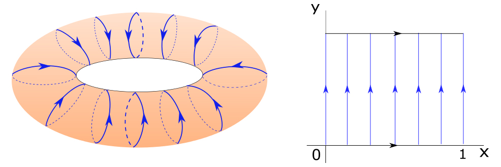
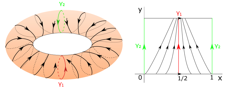
**Figure:** Approximation of a non-Morse-Smale vector field.

We will approximate this non-Morse Smale field by the Morse-Smale vector field $Y$ with two closed orbits: an attractor $\gamma_1$ and a repellor $\gamma_2$.

**Figure:** Approximation of a Morse-Smale vector field.

The two vector fields $X$ and $Y$ can be expressed as: $$X = \cfrac{\partial}{\partial y}$$ $$Y \approx X_{\varepsilon} = \cfrac{\partial}{\partial y} + f_{\varepsilon}(x)\cfrac{\partial}{\partial x}$$ Here, the function $f_{\varepsilon}(x)$ statisfies:

$f_{\varepsilon}(x)=0$ for $x=0, \cfrac{1}{2}$ and $1$
$f_{\varepsilon}(x)>0$ for $x \in (0,\cfrac{1}{2})$
$f_{\varepsilon}(x) <0$ for $x \in (\cfrac{1}{2},1)$

One example of $f_{\varepsilon}(x)$ is: $f_{\varepsilon}(x) = \varepsilon \sin(2\pi x) \text{ for } x \in [0,1]$. Since the norm of this function is less than $1$, $|f_{\varepsilon}(x)|<\varepsilon$ and $|f'_{\varepsilon}(x)|$ is small.

Approximating a General Rational Flow

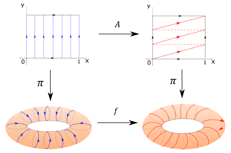
In general, a rational flow on $T^2$ may not be simple like the previous example. Fortunately, there is a way to to reduce any rational flow to the one in this example. Any vector field that induces a rational flow on $T^2$ has an infinite number of closed orbits. Visually, if we can take each closed orbit and convert it into a closed orbit as in the last example, then the two vector fields are topologically equivalent, and the remaining task to approximate that field by a Morse-Smale field becomes simple.
The previous rational flow in $\mathbb{R}^2$ is $X = \begin{cases}{\dot{x}=0\\ \dot{y}=1}\end{cases}$The general rational flow in $\mathbb{R}^2$ is $Y = \begin{cases}{\dot{x}=1\\ \dot{y}=\alpha}\end{cases}$ where $\alpha=\cfrac{m}{n}$ and $m,n \in \mathbb{Z}$ and are relatively prime. We can write these two vector fields on $T^2$ as $X =\cfrac{\partial}{\partial y} $ and $X_\alpha = \cfrac{\partial}{\partial x} + \alpha\cfrac{\partial}{\partial y}$ respectively. They both have infinitely many non-hyperbolic closed orbits on $T^2$. We define the projection map $\pi: \mathbb{R}^2 \rightarrow T^2$ as a quotient map that takes a point $p \in \mathbb{R}^2$ to its equivalence class in $T^2$. Each orbit of $X$ has period of 1 and each orbit of $X_\alpha$ has period of $n$ and goes around the torus $m$ times. Consider the matrix: $ A = \begin{bmatrix} a & n\\ b & m\\ \end{bmatrix}$, where $a$ and $b$ are integers such that $am - bn =1$. Since $\det A=am-bn=1$, $A$ is invertible. We have
$$ AX = \begin{bmatrix} a & n\\ b & m\\ \end{bmatrix} \begin{bmatrix} 0 \\ 1 \end{bmatrix} = \begin{bmatrix} n \\ m \end{bmatrix} = n \begin{bmatrix} 1 \\ \cfrac{m}{n} \end{bmatrix} = nX_\alpha$$ For any vector $v = \begin{bmatrix} x \\ y \end{bmatrix}$ where $x,y \in \mathbb{Z}$, we have $$Av = \begin{bmatrix} a & n \\ b & m \end{bmatrix} \begin{bmatrix} x \\y \end{bmatrix} = \begin{bmatrix} ax+ny \\ bx+my \end{bmatrix}$$ $$A^{-1}v = A^{-1} \begin{bmatrix} x\\y\end{bmatrix}=\cfrac{1}{\det A} \begin{bmatrix} m &-n\\ -b & a \end{bmatrix}\begin{bmatrix} x\\y\end{bmatrix}$$ $$=\begin{bmatrix}m &-n\\ -b & a \end{bmatrix}\begin{bmatrix} x\\y\end{bmatrix} = \begin{bmatrix} mx-ny\\-bx+ay \end{bmatrix}$$ Both $A$ and $A^{-1}$ map integer vectors to an integer vectors. We then define a map $f:T^2 \rightarrow T^2$ by $f(\pi(p)) = \pi(Ap)$. It can be shown that $f$ is a diffeomorphism.

**Figure:** A map beween the "nice" rational flow $X$ nd the general flow $X_\alpha$.

We also have the following propositions

Let $\varphi_t$ and $\psi_t$ be the flows of $X$ and $Y$ on $M$ respectively and $f:M \rightarrow M$ a diffeomorphism such that $f_*(X)=Y$, then $$f(\varphi_t(p)) = \psi_t(f(p))$$ for all $p \in M$, i.e., $f$ is a topological conjugacy.

If $\psi_t$ is the flow of $Y$, then $\psi_{\lambda t}$ is a flow of $\lambda Y$ where $\lambda \in \mathbb{R}$. That is, if $\gamma(t)$ is an orbit of $Y$, then $\gamma(\lambda t)$ is an orbit of $\lambda Y$.

The process of converting $Y$ to $\lambda Y$ is called a reparametrization of $Y$. Since $f_*=A$, $f_*(X)=nX_\alpha$. Let $\varphi_t$ and $\psi^\alpha _t$ be the flows of $X$ and $X_\alpha$ respectively. By the two previous Propositions, the flow of $nX_\alpha$ is $\psi_{nt}^\alpha$, and for all $p \in T^2$, $$f(\varphi_t(p)) = \psi^\alpha _{nt}(f(p)).$$ This means that $f$ takes the orbits of $p$ in $X$ to the orbits of $f(p)$ in $X_\alpha$. However, $f$ does not preserve the period and therefore, $f$ is a topological equivalence, not a topological conjugacy.
The final step is to find a Morse-Smale approximation of the general rational flow $X_\alpha$}. Let $\varepsilon > 0$ be arbitrary, there exists a Morse-Smale vector field $Y$ such that $$\lVert Y-X \rVert_{C^1} < \varepsilon.$$ $$\lVert f_*(Y)-f_*(X)\rVert_{C^1} < c\varepsilon,$$ for some number $c$ depending only on $m$ and $n$. Since $f_*(X)= nX_\alpha$ and $\cfrac{1}{n}f_*(X) = X_\alpha$, $$\lVert\cfrac{1}{n}f_*(Y)-X_\alpha\rVert_{C^1} < \cfrac{c}{n}\varepsilon,$$ The vector field $Z = \cfrac{1}{n}f_*(Y)$ is $C^1$-close to $X_\alpha$ and $Z$ is Morse-Smale because $f_*(Y)$ is the pushforward of the Morse-Smale field $Y$. Thus, $Z$ is a Morse-Smale approximation of the general rational flow field $X_\alpha$.

Conclusion

In dimension two, Morse-Smale systems are structurally stable and form a dense open set as we have seen in the previous sections. With those qualities, we can always approximate a non-Morse-Smale field by a Morse-Smale field. Although we only showed a few simple examples in $S^2$ and $T^2$, some of these properties can be generalized to more complicated cases. For example, the Closing Lemma shows that Morse-Smale systems are dense in $\mathfrak{X}^1(M^2)$, whether $M$ is orientable or not. Besides $S^2$ and $T^2$, there are also studies that show the same results for the projective plane $P^2$ and the Klein bottle $K^2$. However, in dimension three or higher, Morse-Smale systems are not dense. In these manifolds, there are also structurally stable systems that are not Morse-Smale. Some of these systems have infinitely many closed orbits. This implies that Morse-Smale systems cannot be used to approximate all vector fields in higher dimensions. In discrete dynamical systems, there are also non-Morse-Smale systems that cannot be approximated by Morse-Smale ones. In recent years, Morse-Smale systems have been generalized to the discrete setting and used in the field of topological data analysis.